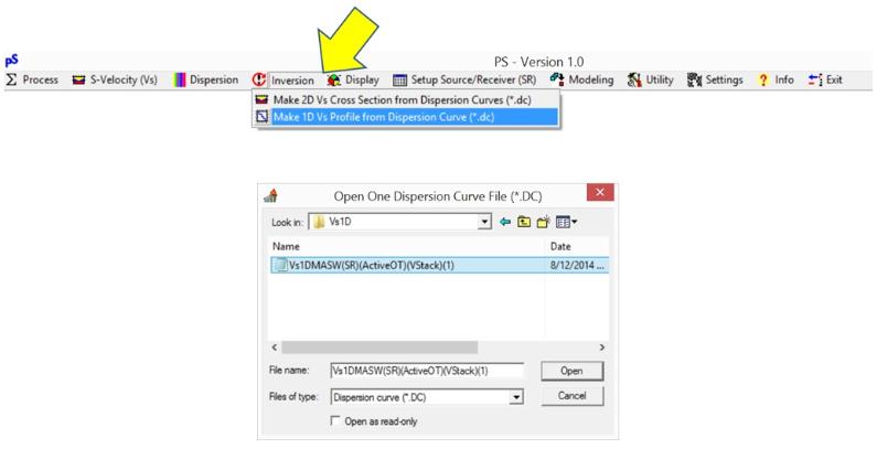
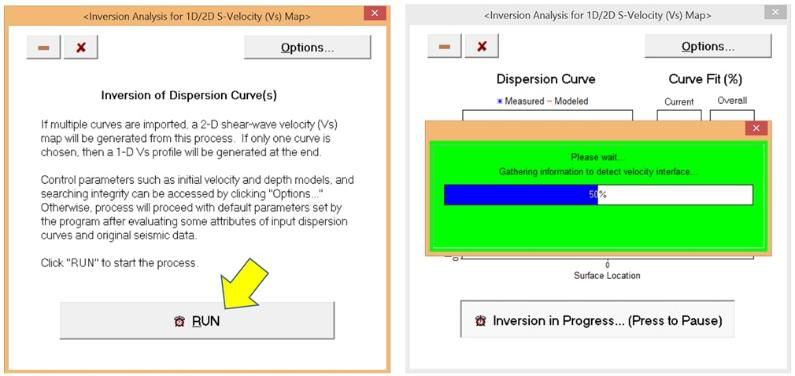
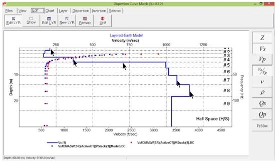
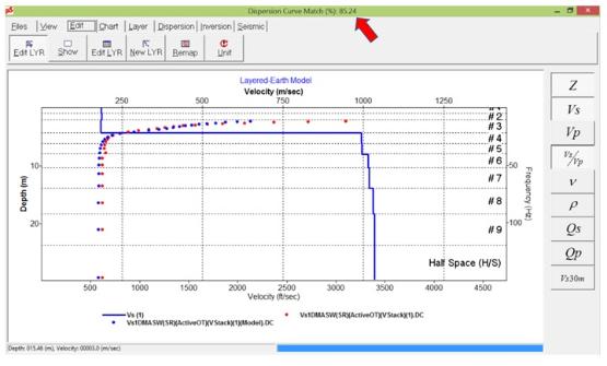
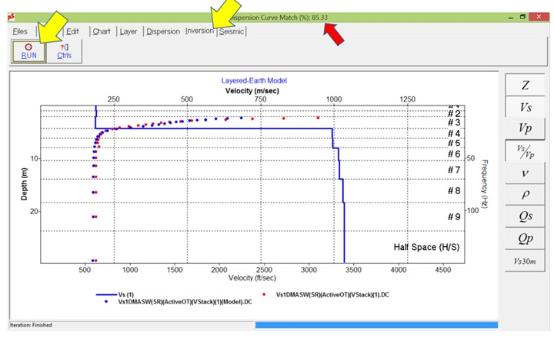
Now, because the "initial" velocity model has been slightly updated, another automatic inversion may find "further improved" velocity profile. So, it is now attempted to run it again by selecting "Inversion" tab on the menu panel, and then clicking "RUN" button as illustrated below. The new match (85.33 %) now shows it little improved. This is usually the case if the new automatic inversion process could not find another model significantly different from current one that maintains comparable or improved match in M0 curves.
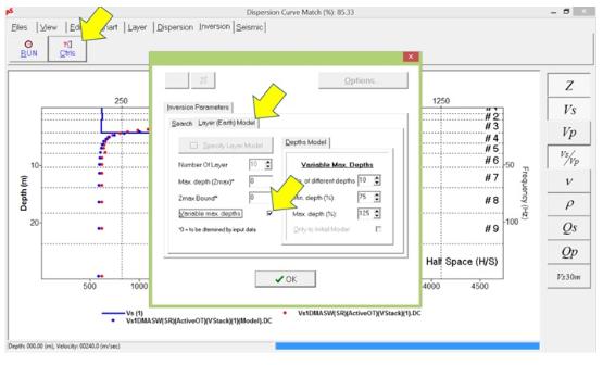
Then, it is worthwhile trying to introduce another degree of freedom in the process by choosing the option of "Variable max. depths" as illustrated below. It will then execute the automatic inversion process for as many different depths models as selected (e.g., 10) that are created by either contracting (< 100 %) or stretching (> 100%) current velocity model. The example illustrated below indicates that the process will examine ten (10) different initial models within 75% - 125% scale of current velocity model. From the search with all these different models, the program will show at the end the model that has the best (i.e., highest) match.
Click "Run" button to perform this "Variable max. depths" inversion. After a while, the final solution of velocity model will be displayed. The example below indicates the match improved noticeable from 85.33% to 89.34%. Above all, the profile looks quite realistic.
Now, it may be the time to save it as the final solution.

