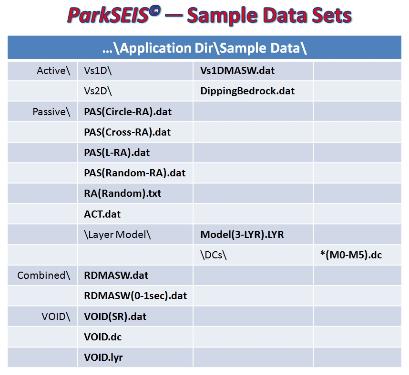
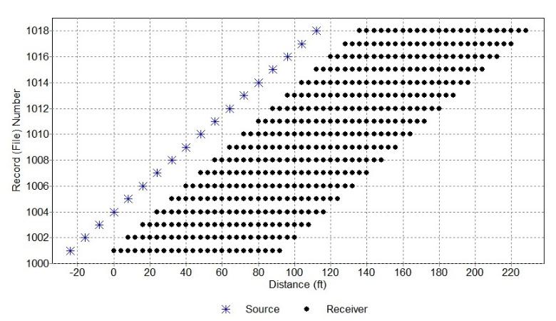
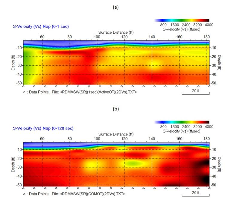
Download synthetic and real data sets (#1 and #2) for AUTO process demonstration. They are not counted as "usage" of AUTO module. All these data sets already have source/receiver (SR) setup encoded [*(SR).dat]. When testing, therefore, select "Seismic Data with Source/Receiver Coded" option by going to "AUTO" -> "2D S-Velocity Cross Section From" in the main menu.
Sample Data Sets in ParkSEIS
See user guide and watch video tutorials ("About Sample Data" and "Processing Sample Data")
Active Survey Data Set
There are two different types of active data sets; one that is used to generate a 1-D Vs profile ["SampleData(Vs1D).dat"] and another to produce a 2-D Vs cross section ["SampleData(Vs2D).dat"]. The entire procedures of data analysis using these two data sets are explained in separate user guides of "Generating 1-D Profile (Working with Sample Data)" and "Generating 2-D Cross Section (Working with Sample Data)",
Passive Survey Data Set
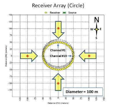
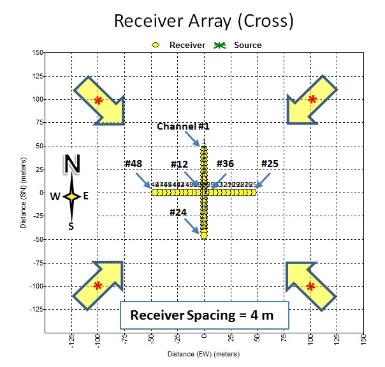
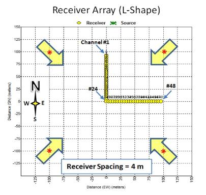
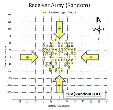
Four (4) passive survey data sets are provided that were recorded using four (4) different types of 2-D receiver arrays (RA's)—circle ["...\PAS (Circle-RA).dat"], cross ["...\PAS(Cross-RA).dat"], L shape ["...\PAS(L-RA). dat"], and random ["...\PAS(Random-RA).dat"]. A passive data set recorded using a 1-D (linear) receiver array is considered identical to the data set from the active/passive combined survey described below.
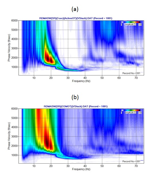
The data analysis procedure is demonstrated from source/receiver (SR) setup to dispersion imaging steps, while the remaining steps will be identical to those demonstrated in the active data sets. Because the most common way of utilizing passive data is to provide useful dispersion information at such low frequencies where active data usually does not provide objective dispersion trends, it is also demonstrated to combine the passive and active dispersion images. All passive data sets are synthetic (model) data created by using the reflectivity modeling module included in the main menu [see the user guide "Modeling (Seismic Data)"]. A 48-channel acquisition of relatively short recording time (T≈8 sec) with a 4-ms sampling interval (dt) was used during the modeling. Although the actual recording time for a passive survey will be usually much longer than this (for example, T = 30 sec), the short recording time was due to the limitation in the modeling module. Generation of surface waves (from 5 to 100 Hz) was simulated during the modeling by placing multiple (4) active source points at a certain distance (i.e., approximately the same distance as the dimension of the receiver array) away from the 2-D RA distributed along the full 360-degree azimuth range with an equal interval of 90 degrees as shown in Figures 1-4. Excitation time of each source point was modeled with a 2-sec interval between the two successive points (for example, 1- sec, 3-sec, 5-sec, and 7-sec for source points at 0 degrees, 90 degrees, 180 degrees, and 270 degrees, respectively). This azimuth and source excitation time information is obtained as by-products during the dispersion imaging process by Park (2010) (see the user guide "Dispersion Image Generation" for more details). How to display this information after generation of the dispersion image from the passive data set is also demonstrated.


