1. Importing Input Data - Dispersion Curves (*.dc)
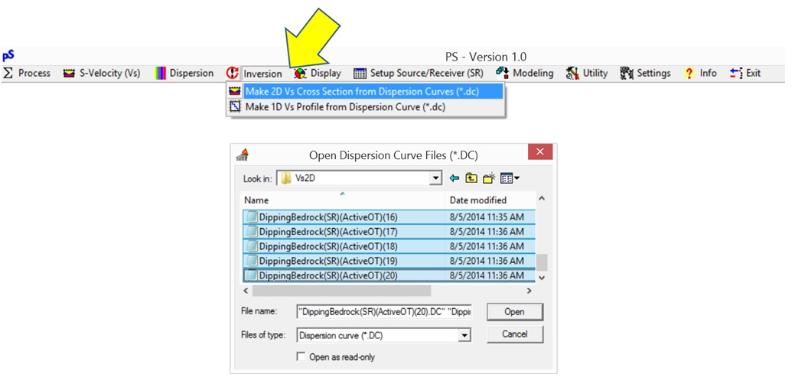
To generate a 2-D (depth and surface distance) shear-wave velocity (Vs) cross section, go to "Inversion" → "Make 2D Vs Cross Section from Dispersion Curves" and select multiple dispersion-curve (*.DC) files at the same time that were previously prepared by analyzing a data set from the same (one) survey line.
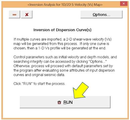
Then, the following dialog will be displayed to confirm the maximum depth (Zmax) of the inversion that is originally determined by the program based on the average offset range used during data acquisition. This is one of the most important parameters in inversion process that is directly related to the resolution of the final 2-D shear-wave velocity (Vs) map. If you click "No", then the program will show the relevant tab where you can adjust Zmax as well as other parameters. Otherwise, click "Yes."
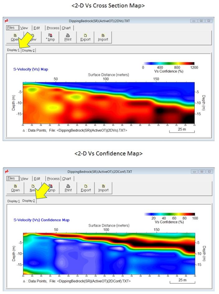
At the end of the inversion process, the following two types of output will be saved and then automatically displayed within the same form (under "Display 1" and "Display 2" tabs); a 2-D shear-wave velocity (Vs) cross section map [*(2DVs).TXT], and corresponding 2-D Vs confidence map [*(2DConf).TXT], respectively, as shown below. Velocity color scheme in the 2-D Vs cross section is automatically determined by the program based on the velocity value distribution in the input file [*(2DVs).TXT] and this can be changed through a control dialog explained below. It can be noticed that the cross section map shown below used the color scheme displayed on top that is matched within the Vs range of 0-1200 m/sec. The confidence map shows distribution of relative reliability in inversion results (Vs values) so that it can be used to judge credibility of velocity values in cross section map that may change from one place to another.


