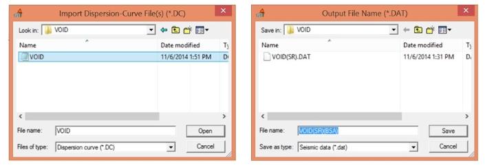
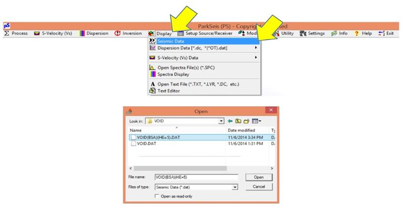
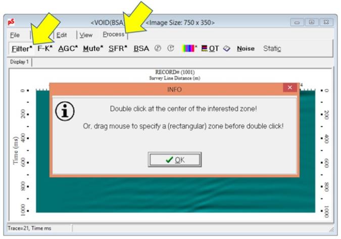
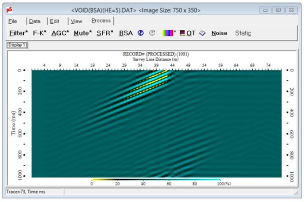
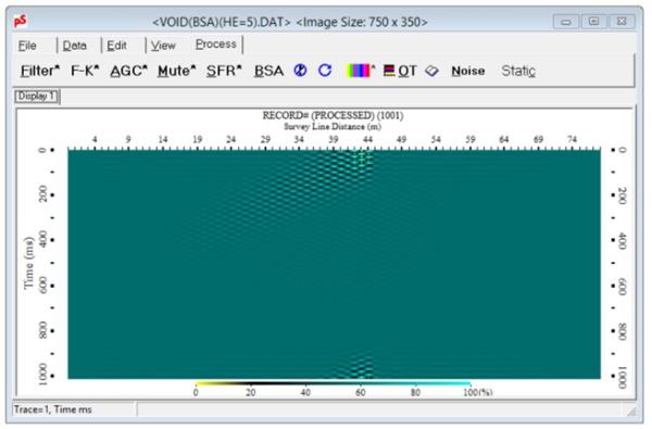
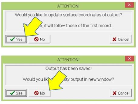
After this, the BSA operation will be executed and the final BSA section will be displayed. Default display mode for BSA section is a variable-area display as shown below. The target back scattering feature originating from the surface location of the anomaly (44-m) is indicated in the figure below. All other less conspicuous slant features are computational artifacts.
4. Generating Average Dispersion Curve
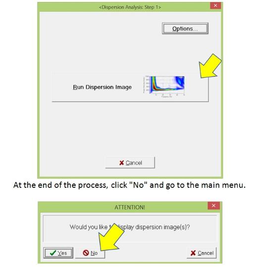
This section describes how to prepare one dispersion curve that represent the average dispersion property over the entire surveyed distance. Although you can import all the dispersion curves processed from all the records in the input seismic data set, the most optimal BSA output is often generated when this "representative" dispersion curve is used for the process. This section will demonstrate how to generate all individual dispersion images from the sample data set (of 50 records). Then, they will be stacked to produce one "stacked" dispersion image, from which the representative dispersion curve will be extracted and saved to be imported at the beginning of the BSA process.
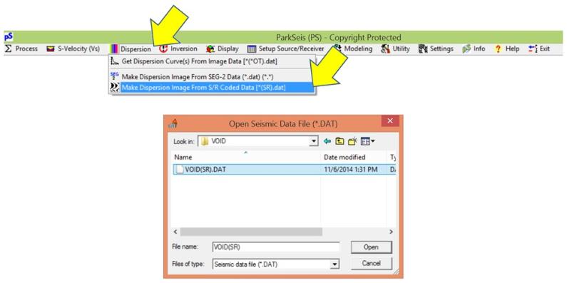
In the main menu, go to "Dispersion" → "Make Dispersion Image From S/R Coded Data" and import the same data set [VOID (SR).DAT].
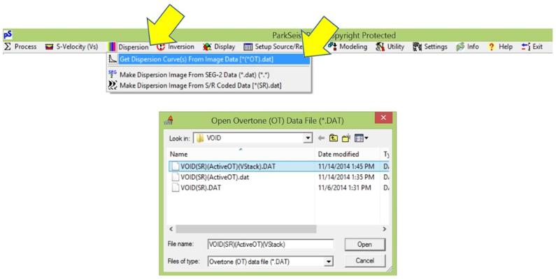
Then, in the main menu, go to "Dispersion" → "Get Dispersion Curve(s) From Image Data" and import the previously saved stacked image [*(VStack).DAT].
The following display window in which you can extract the dispersion curve from the image will appear. Although detailed instructions about how to extract a dispersion curve from the dispersion image is explained in the user guide of "Dispersion Curve Extraction (Vs1D)" [or "*(Vs2D)"], the simplest sequence would be, first, click the "Bounds" button and then click several points (e.g., five or more) on the dispersion trend to mark the lower and upper bounds within which the curve will be extracted based on the maximum amplitude at each frequency. Then, click the "Extract" button to extract the curve shown in the image below. Click "Save" button to save the extracted curve (*.DC). This is the "average" dispersion curve that is representative of the entire survey area and you can import it during the BSA operation.


