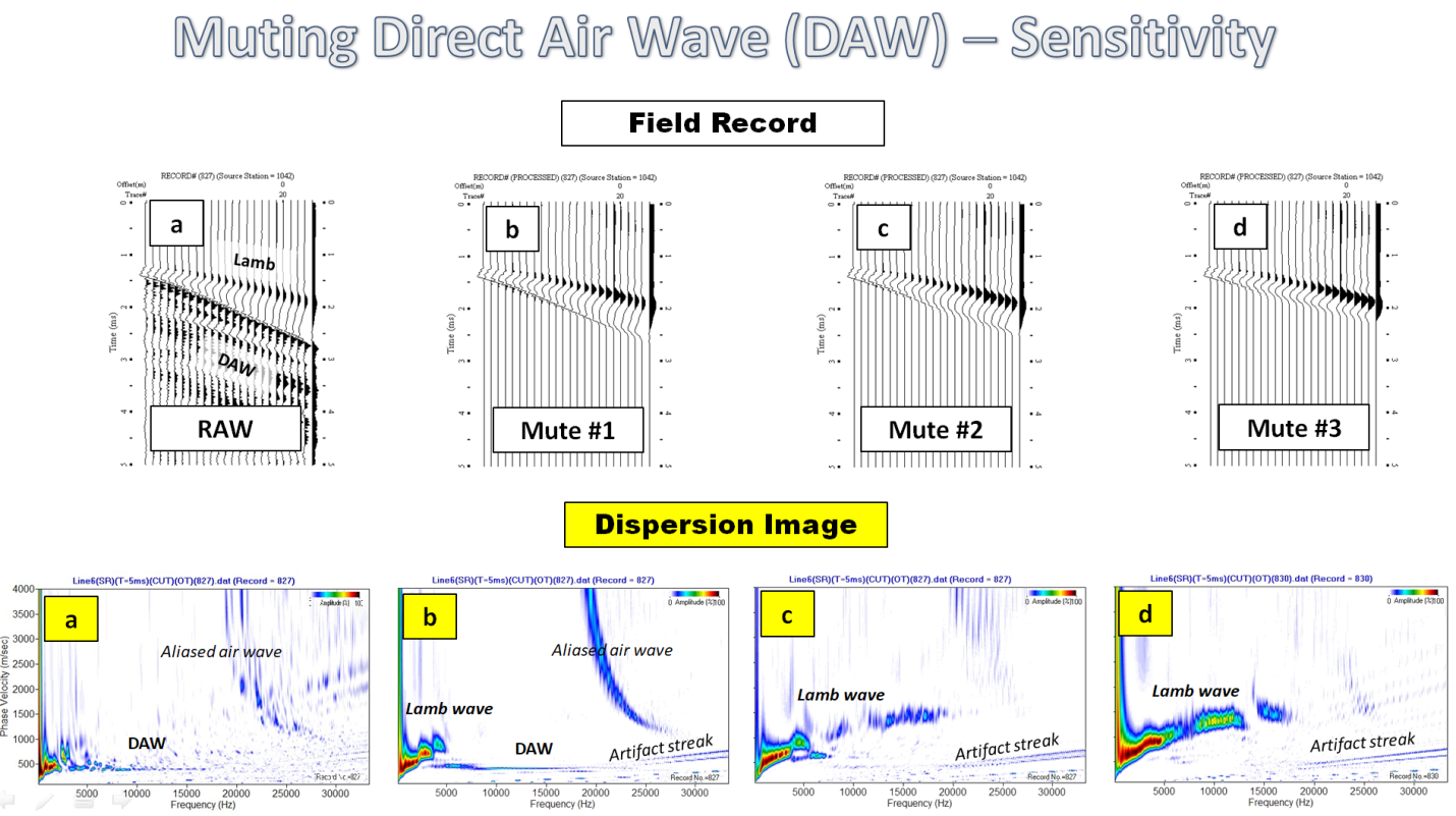
General procedure of data analysis is similar to the common MASW procedures of dispersion and inversion for the pavement (Ryden et al., 2004). However, there is a critical pre-processing step, without which all the subsequent steps become useless. It is the step to curtail (“mute”) the amplitude of direct air wave (DAW) arrivals.
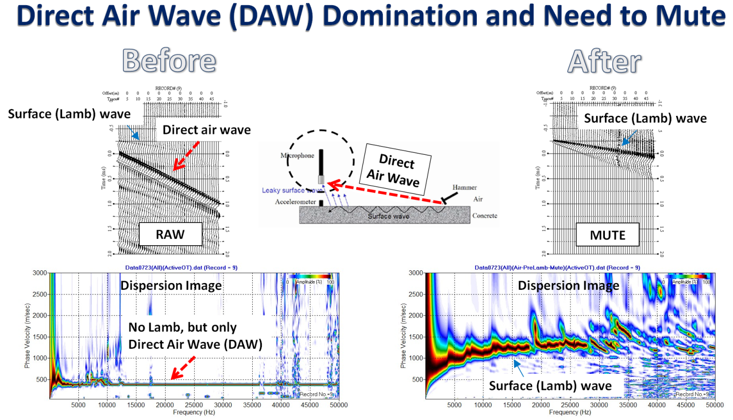
Two approaches can be used for the DAW muting process; manual and automatic processes. The former requires the operator to manually identify the optimum muting parameters (e.g., start time and slope) and specify it on the displayed record using mouse one by one. This is not convenient and requires skillful experience. The latter employs the prediction of the DAW arrival time based on a common sound speed (e.g., 340 m/s) and the triggering mechanism of the recording device (e.g., triggered by a certain voltage in the 1st channel that can be either DAW or Lamb wave amplitude). Although this approach can be fully automated, it can also introduce significant uncertainties because of the inconsistent waveform in the triggering wave type (DAW or Lamb). The most robust automatic process must be based on the linear-move-out (LMO) semblance analysis of acquired raw record that can reveal the velocity (V-air and V-Lamb) and arrival time (t0-air, t0-Lamb) of DAW and Lamb wave, both of which may change from one record to another slightly (e.g., ±0.5 ms). This “slight” change in arrival time can be significant enough for the purpose of muting DAW properly because the arrival time difference between the two types of waves is only in 0.5 ms – 1.5 ms range.
Once the raw record is properly muted in DAW, it goes into the dispersion image construction by using the 2D wavefield transformation method of Park et al. (1999), from which a dispersion curve is picked in a broad frequency range (e.g., 100 Hz – 30,000 Hz). The low-frequency portion (e.g., 100 Hz – 500 Hz) is inverted using the general Rayleigh wave algorithm, while the remaining high-frequency portion is inverted based on the Lamb-wave algorithm. This inversion process generates a 1D shear-wave velocity (Vs) profile with a depth 60% of the array length (e.g., 0.3 m). All these analysis steps are fully automated without any need for operator’s involvement in the ParkSEIS-X (PSX) software package.